Plot Panel¶

The Plot Panel visualizes your signal data as interactive time-series charts. It is designed for timeline-driven analysis with zooming, cursor control, and precise measurement tools.

Overview¶

The plot panel displays signals as line charts with time on the x-axis and signal values on the y-axis. Each signal gets its own color and can be toggled on/off individually. The panel supports real-time streaming data and historical analysis.

Basic Usage¶

Adding Signals¶

Drag and drop signals from the signal tree directly onto the plot panel. Each signal will appear as a colored line with a legend entry.

Left-drag to select a range and zoom into that time window
Double-click to step back one view state (zoom/history reset behavior)
Right-click to set the shared timeline cursor at the clicked timestamp
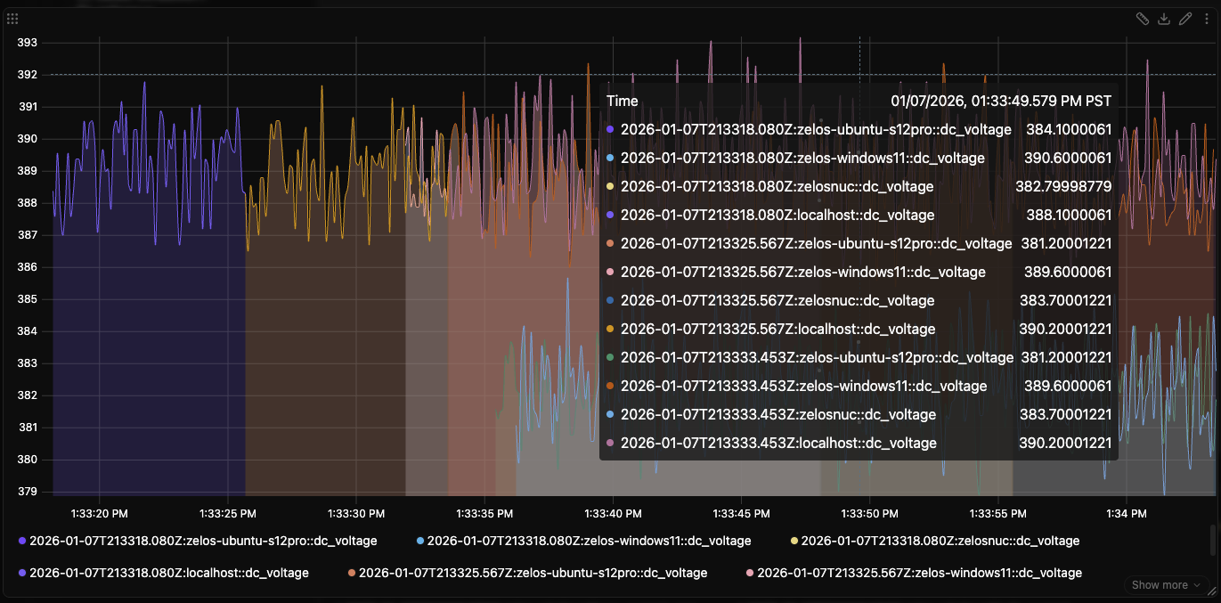
Hover to inspect nearest signal values in the tooltip

Signal Management with Signal Chips¶

Below the plot, each signal is represented by an interactive signal chip that provides comprehensive signal management:

Color Management¶

Color indicator - Colored circle showing the signal's current plot color
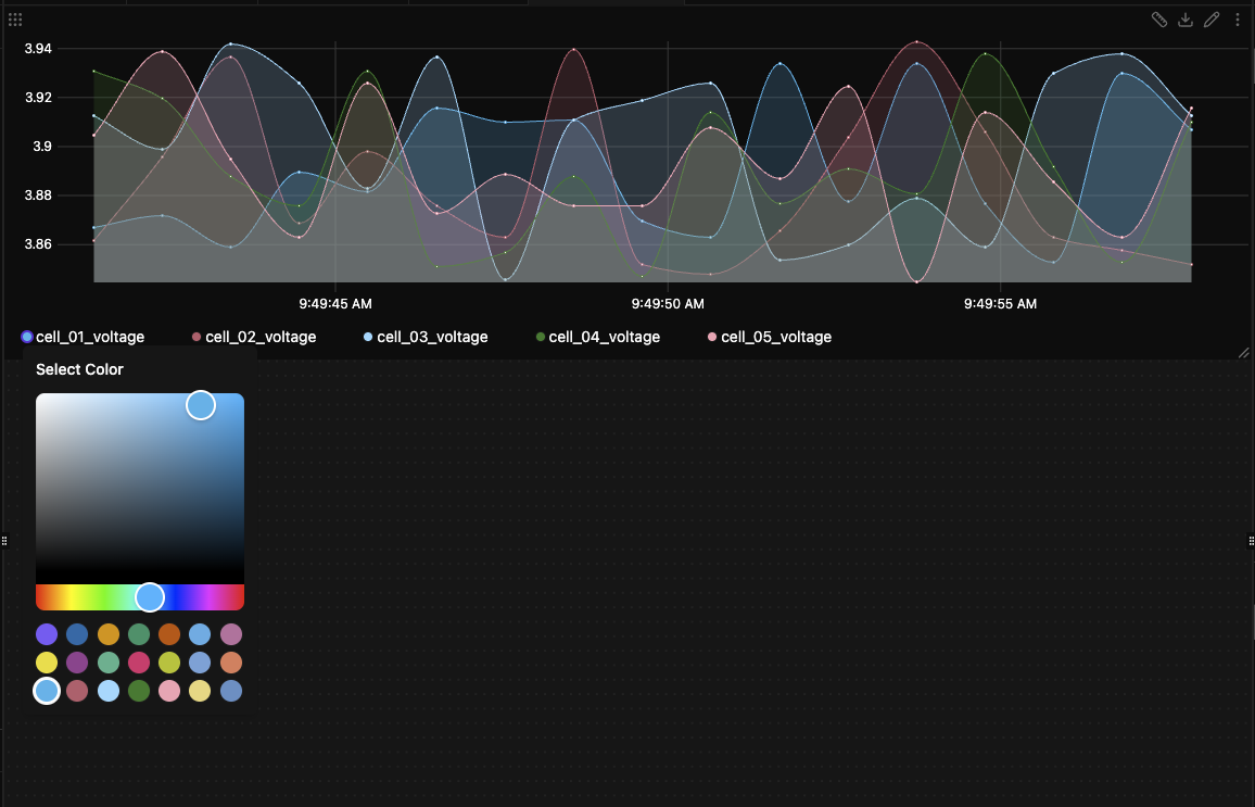
Color picker - Click the color circle to open a color picker (see Color System below)
Visual states - Solid circle when active, hollow circle when hidden

Signal Control¶

Toggle visibility - Click anywhere on the chip to show/hide the signal line
Remove signal - Click the X button to remove from the panel entirely
Drag to other panels - Drag chips between panels to reorganize your data

Information Display¶

Signal name - Shows full path or shortened name based on panel settings
Data type - Hover to see signal data type in tooltip
Status indicator - Muted when the signal has no data in the current view (see Show Empty Signals)

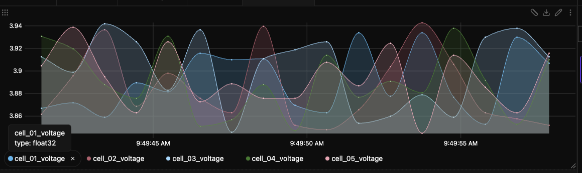
Signal Management — Signal chips for managing individual signals in the plot.

Show Empty Signals¶

Edit Panel -> Config -> Show empty signals (on by default) keeps a configured signal's legend chip even when it has no samples in the current view.

On: the signal keeps a muted chip even with no line drawn.
Off: only signals with data in the current view appear in the legend.

Muted chips come in two kinds:

Empty -- plain muted. The signal has no samples in the current view; the chip tooltip reads No data in this time range. Zoom or scroll the timeline back over its data and the chip becomes colored again.
Unavailable -- muted with an unplug icon. The signal's source is offline or its path was not found. The tooltip gives the reason, such as Source robot disconnected, Source drive.trz closed, or Not found in any connected source.

The default for new panels is set in Settings -> General -> Panel Defaults.

Color System¶

Click the color circle on any signal chip to open the color picker:

Visual color selector - Interactive gradient picker for precise color selection
Quick palette - 20+ pre-selected CVD-safe colors for fast selection
Real-time preview - Colors update smoothly while dragging in the selector

Color Behavior and Stability¶

Plot colors are assigned per logical signal path and scope, then preserved as you work:

Changing a signal color from the chip or from Edit Panel -> Data updates the plotted series immediately
Portable signals use their configured chip color as the base color for matching series
When one logical signal expands across multiple traces and/or agents, each scope keeps its own color so matching sources stay distinguishable
Recoloring one scoped variant does not recolor sibling traces/agents, and removing one signal does not force the remaining series to pick new colors
Stored colors survive editor open/close, tab switches, app reloads, and saved layout/workspace restore as long as the signal binding still exists

Display Format¶

Right-click any signal chip below the plot to change how that series's values are displayed in the tooltip and the measurement tool. The menu offers five formats: Default, Hex, Binary, Octal, and Scientific. The same menu can copy the signal path, and can copy the current value when data is available. The same formats are available from Edit Panel -> Data -> the per-row ellipses menu.

Formats are stored per panel and per series: the same signal placed in two plots can render values as 0xFF in one tooltip and 255 in the other. When a signal is scoped or expanded into multiple series (multi-producer or overlapping-segment cases), each series keeps its own format. Formats travel with the chip on panel-to-panel drag-and-drop, and survive scope changes, reload, and workspace save/load.

Hex / Binary / Octal apply to integers directly. For floats, integer-valued floats (like 42.0) render in the short form (0x2A); other floats render the IEEE 754 64-bit bit pattern (for example, 3.14 becomes 0x40091EB851EB851F). Dictionary-encoded signals only support the default label rendering, so non-default kinds are greyed out in the picker. If a signal has a value-table mapping (for example, 1 -> "Run"), the label is preserved alongside the formatted raw: Run (0x1) instead of just 0x1. The chip itself never changes appearance when a format is set: the cell text and tooltip are the only state indicators.

The Y-axis tick labels intentionally stay in the default base-10 format regardless of any per-series format. Plots commonly mix signals with different formats (or have no user-set format at all), and Y-axis ticks land on non-integer scale values that would be meaningless as IEEE bit patterns — the axis is treated as a shared reference scale so cursor-reported values (tooltip, measurement tool) are the only surfaces that adopt the chosen format.

Legend Layout¶

Plot legends can sit below the chart or beside it:

Bottom - Compact rows below the plot (default)
Left - Vertical legend on the left side
Right - Vertical legend on the right side

Use Edit Panel -> Display to change placement. The legend includes a resize handle so you can tune how much space is reserved for signal names versus chart area.

Multi-Trace Plotting¶

The plot panel supports viewing signals from multiple traces simultaneously, enabling powerful comparison and analysis workflows.

Viewing Multiple Traces¶

Add signals from different traces to the same plot panel to compare data across recordings:

Trace identification - Each signal shows its source trace in the legend for clear identification
Agent labels - Signals display both trace and agent information when needed

Multi-Trace Plot — Multiple traces displayed on a single plot with clear identification.

Timeline Cursor Integration¶

The plot panel is fully synchronized with the global timeline cursor used by table, value, and log panels.

Right-Click to Jump Cursor¶

Right-click anywhere in the plot area to jump the shared timeline cursor to that timestamp.

In paused mode, this updates cursor time in-place.
In live mode, this action transitions to paused view and sets the cursor to your clicked time.
All other timeline-aware panels immediately sync to the new cursor position.

Dragging the Plot Cursor¶

When paused (and playback is not running), the plot renders a draggable cursor handle:

Drag horizontally to scrub exact cursor time directly from the plot
Cursor movement updates the global timeline cursor in real time
Handle is hidden while playback is actively running

Values in the Legend¶

While paused, each legend chip shows its signal's value at the timeline cursor. Pausing places the cursor at the right edge of the view, so the readout appears immediately — and it follows every scrub, right-click jump, and playback tick from there. Values resolve with the same left-closest semantics as the tooltip (the value the signal held at the cursor time); a — means the signal has no sample at or before the cursor. Hover a chip to see the full value with its sample time.

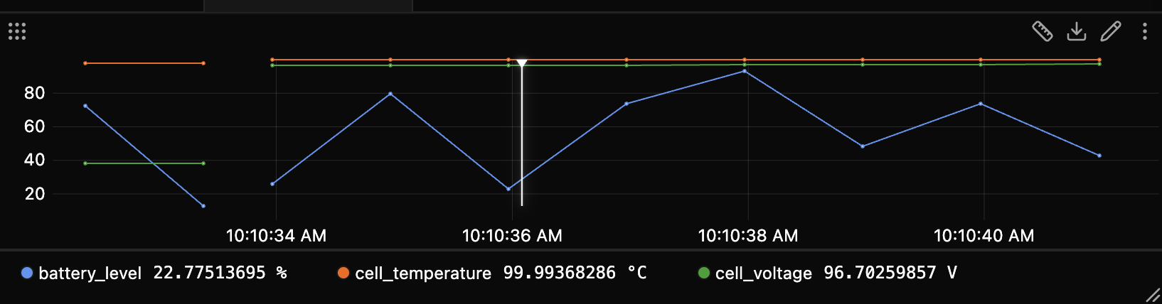
Paused plot with the timeline cursor set and each legend chip showing its signal's value at the cursor — Paused — each legend chip reads out its signal's value at the timeline cursor.

In live mode, Edit Panel -> Config -> Live values (off by default) streams each signal's latest value into its chip instead. The default for new panels is set in Settings -> General -> Panel Defaults.

While the measurement tool is active, the chip slot shows the signed Δ between the two measurement cursors in place of the cursor value.

The state panel's legend chips read out the same way, showing each signal's state label at the cursor (or the latest state in live mode with Live values on).

The cursor lookup uses left-closest behavior:

Tooltip values resolve to the closest sample at or before the hovered time
If a hovered point is null, lookup backtracks to the nearest earlier non-null sample
This avoids misleading forward jumps when data is sparse or gapped

Zoom and View History¶

Zoom and reset behavior in the plot panel is stateful and mode-aware:

Drag-selecting a time range commits a zoom step
Double-click steps back through zoom/view history
If no history remains:
live workspaces return to live follow
trace/paused workspaces return to the initial paused view window
Starting a new drag-select while playback is running stops playback first

Measurement Tool¶

The measurement tool allows you to make precise measurements between two points on your signals. This is particularly useful for analyzing signal deltas, timing relationships, and precise value changes.

Plot measurement: two cursors with a Δt span bracket between them and a signed Δ on each legend chip — Measuring on a paused plot — cursor 1 (blue) at the earlier time, cursor 2 (green) at the later time, the Δt span bracket between them, and each signal's signed Δ on its legend chip.

Activating Measurements¶

Pause the view - The measurement tool is disabled in live mode
Click the ruler icon in the panel header to toggle measurement mode on
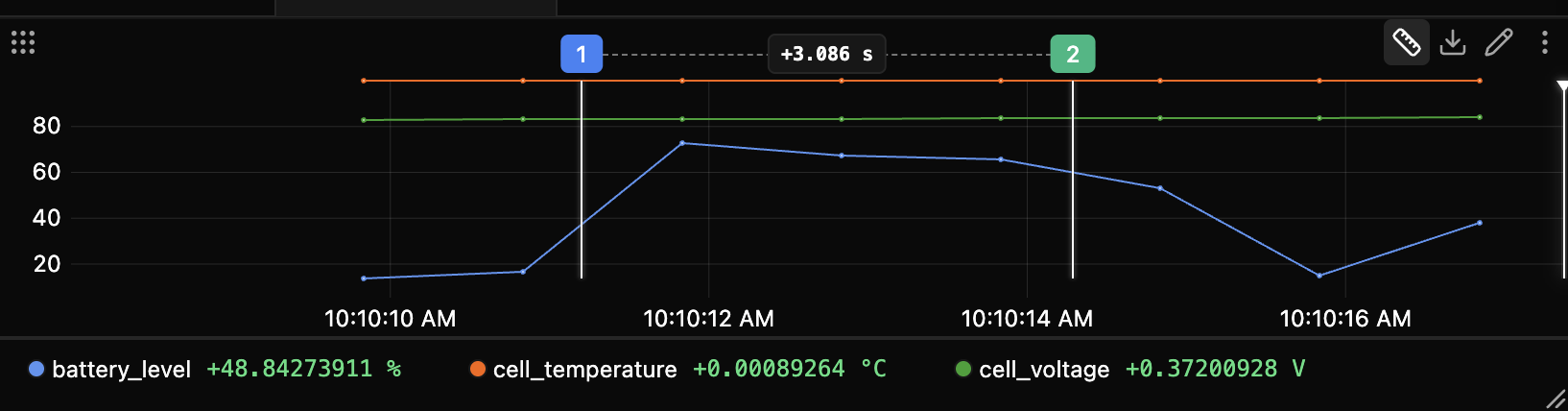
Both cursors are placed automatically - Like an oscilloscope, enabling the tool drops both cursors at once, at roughly 1/3 and 2/3 of the current view
Read the results in place - The time difference Δt appears as a span bracket between the two cursors, and each visible signal's value change shows in the legend (see Measurement Results)

From there, drag either cursor to fine-tune the span — there is no separate click-to-place step.

Pause Required

The measurement tool is only available in paused mode. If you try to activate it while in live mode, you'll see a tooltip indicating you need to pause first.

Legend Reveals Itself

The per-signal deltas live in the legend, so if the legend is hidden it is automatically shown while you measure, then restored to hidden when you toggle the tool back off.

Using Measurement Cursors¶

The two cursors are placed for you when you enable the tool; from there they are fully interactive:

Adjusting Cursors¶

Drag the cursor line to reposition it
Drag the numbered label (1 or 2) for an easier grab target
Cursors snap to the nearest data point as you drag
If you drag one cursor past the other they automatically swap, so Cursor 1 (blue) always stays at the earlier time and Cursor 2 (green) at the later time

The hover tooltip keeps working while the measurement tool is active, reporting each signal's value at the hovered time. It is suppressed only while you are actively dragging a cursor, then returns as soon as you release.

Toggling the ruler drops both cursors at once; dragging either one updates the Δt bracket and every legend Δ live:

Measurement Results¶

Results are shown in place — directly on the plot and in the legend.

Time delta (Δt)¶

The time difference between the two cursors is drawn as a span bracket between them, directly on the plot. It uses the standard delta format (auto-selected s/ms/µs/ns units), so the labelled span always lines up with the timeline.

Per-signal value change (in the legend)¶

Each visible signal reports its value change Δ (End − Start) on its own legend chip, signed and color-coded — green for an increase, red for a decrease:

In a left or right legend, the Δ is a right-aligned value column beside each signal name
In a bottom legend, the Δ is an inline token on the signal's pill
Hover any chip to see that signal's exact start → end values in its tooltip

Because the legend already lists every signal with its color and name, the delta simply rides along on the chip — there is no extra panel or table to manage.

Visible Signals Only

Only currently visible signals get a Δ. Signals hidden via their signal chip show no delta.

Measurement Data Formats¶

Time¶

Δt uses the delta format — signed, with automatic s/ms/µs/ns units based on magnitude

Values and deltas¶

Per-signal values use the same formatter as the tooltip and table: your per-series display format (Default, Hex, Binary, Octal, Scientific), units, and value-table / dictionary labels all apply
The Δ is purely numeric and signed (+/−): it keeps the unit but ignores value-table and dictionary mappings, since the change between two labels is not itself a label

Precision¶

Timestamps are stored and calculated in nanosecond precision
Values keep their original signal precision
Each cursor resolves to a real sample, and the delta is computed from those two samples

Plot Panel Settings¶

Access panel settings through the edit panel dialog:

Display Options¶

Panel Title: Set a custom title for the panel. Leave empty to use the default display.

Display Full Name: Toggle between showing full signal paths (source/event.field) or shortened names (field).

Y-Axis Range¶

Control the Y-axis scale to focus on specific value ranges. Access these settings by clicking the edit button in the panel header.

By default, plots auto-scale to show all data. You can override this by setting min/max values:

Min	Max	Behavior
Empty	Empty	Auto-scale to fit all data (default)
`0`	Empty	Fixed bottom at 0, auto-scale top
Empty	`100`	Auto-scale bottom, fixed top at 100
`0`	`100`	Fixed range from 0 to 100

Common Use Cases:

Show zero baseline - Set Min=0, leave Max empty
Logic level monitoring - Set Min=0, Max=3.3 for 3.3V signals
Zoom to range - Set both to focus on a specific value range
Compare plots - Use identical ranges across multiple panels

Tip

Leave both fields empty to return to auto-scaling.

Tips¶

Measurement Accuracy¶

Zoom in closer to your area of interest before measuring, then drag the cursors to fine-tune
Cursors snap to data points as you drag for maximum precision
Zoom in so the cursors snap close to real samples when exact timing matters
Hide irrelevant signals to keep the legend's deltas focused on the signals you care about

Export Data¶

The plot panel supports exporting data in multiple formats:

CSV - Tabular format with timestamps and signal values
JSON - Structured format with metadata and arrays

Exported data respects the current time range and includes all visible signals. Measurement cursors do not affect export scope - the full visible time range is always exported.

Interaction Controls¶

Left-drag - Select a range and zoom
Double-click - Step back through zoom/view history
Right-click - Set shared timeline cursor to clicked time
Cursor handle drag (paused) - Scrub timeline cursor directly in the plot

Data Availability

Measurement accuracy depends on data resolution. With sparse data, each cursor resolves to the nearest sample at or before its position rather than to the exact cursor time. Zoom in to place cursors directly on real samples.